Lecture 05 autograd 与逻辑回归
本节课主要分为两部分:PyTorch 中的自动求导系统以及逻辑回归模型。我们知道,深度模型的训练就是不断地更新权值,而权值的更新需要求解梯度,因此,梯度在我们的模型训练过程中是至关重要的。然而,求解梯度通常十分繁琐,因此,PyTorch 中引入了自动求导系统帮助我们完成这一过程。在 PyTorch 中,我们无需手动计算梯度,只需要搭建好前向传播的计算图,然后根据 PyTorch 中的 autograd 方法就可以得到所有张量的梯度。
1. autograd:自动求导系统
torch.autograd.backward()
功能:自动求取计算图中各结点的梯度。
1
2
3
4
5
6
torch.autograd.backward(
    tensors,
    grad_tensors=None,
    retain_graph=None,
    create_graph=False
)
主要参数:
tensors:用于求导的张量,如loss。retain_graph:保存计算图,PyTorch 默认在反向传播完成后丢弃计算图,如需保存则将该项设为True。create_graph:创建导数计算图,用于高阶求导。grad_tensors:多梯度权重,当我们有多个loss需要计算梯度的时候,就需要设置各个loss的权重比例。
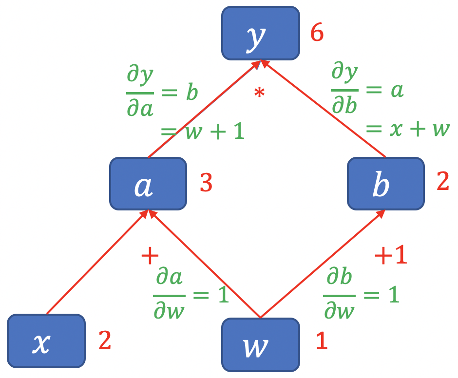
回顾一下如何通过计算图求解梯度:
\[y=(x+w) * (w+1)\]- $a = x+w$
- $b=w+1$
- $y=a*b$
代码示例:
1
2
3
4
5
6
7
8
9
10
11
12
w = torch.tensor([1.], requires_grad=True)
x = torch.tensor([2.], requires_grad=True)

a = torch.add(w, x)
b = torch.add(w, 1)
y = torch.mul(a, b)

# 如果希望后面再次执行该计算图,可以将 retain_graph 参数设为 True
# y.backward(retain_graph=True)

y.backward()
print(w.grad)
输出结果:
1
tensor([5.])
当有多个 loss 需要计算梯度时,通过 grad_tensors 设置各 loss 权重比例:
1
2
3
4
5
6
7
8
9
10
11
12
13
14
15
16
17
18
19
20
21
22
w = torch.tensor([1.], requires_grad=True)
x = torch.tensor([2.], requires_grad=True)

a = torch.add(w, x)
b = torch.add(w, 1)

# y0 = (x+w) * (w+1)    dy0/dw = 2*w + x + 1 = 5
y0 = torch.mul(a, b)

# y1 = (x+w) + (w+1)    dy1/dw = 2
y1 = torch.add(a, b)

# 这种情况下,loss 是一个向量 [y0, y1]
loss = torch.cat([y0, y1], dim=0)

# 梯度的权重:dy0/dw 权重为 1,dy1/dw 权重为 2
grad_tensors = torch.tensor([1., 2.])

# gradient 传入 torch.autograd.backward() 中的 grad_tensors
loss.backward(gradient=grad_tensors)

print(w.grad) # 5*1 + 2*2 = 9
输出结果:
1
tensor([9.])
torch.autograd.grad()
功能:求取梯度。
1
2
3
4
5
6
7
torch.autograd.grad(
    outputs,
    inputs,
    grad_outputs=None,
    retain_graph=None,
    create_graph=False
)
主要参数:
outputs:用于求导的张量,如loss。inputs:需要梯度的张量。create_graph:创建导数计算图,用于高阶求导。retain_graph:保存计算图。grad_outputs:多梯度权重。
求取二阶梯度:
1
2
3
4
5
6
7
8
9
10
x = torch.tensor([3.], requires_grad=True)
y = torch.pow(x, 2)  # y = x**2

# grad_1 = dy/dx = 2x = 2 * 3 = 6
grad_1 = torch.autograd.grad(y, x, create_graph=True)
print(grad_1)

# grad_2 = d(dy/dx)/dx = d(2x)/dx = 2
grad_2 = torch.autograd.grad(grad_1[0], x)
print(grad_2)
输出结果:
1
2
(tensor([6.], grad_fn=<MulBackward0>),)
(tensor([2.]),)
注意事项:
- 梯度不自动清零。
- 依赖于叶子结点的结点,
requires_grad默认为True。 - 叶子结点不可执行原位操作 (in-place)。
代码示例 1:
1
2
3
4
5
6
7
8
9
10
11
12
13
14
15
16
17
18
19
20
21
22
23
# 1. 梯度不会自动清零,重复求取会叠加,可以使用 .grad.zero_() 方法手动清零
w = torch.tensor([1.], requires_grad=True)
x = torch.tensor([2.], requires_grad=True)

for i in range(3):
    a = torch.add(w, x)
    b = torch.add(w, 1)
    y = torch.mul(a, b)

    y.backward()
    print(w.grad)

# 梯度清零,下划线表示原位操作 (in-place)
w.grad.zero_()

for i in range(3):
    a = torch.add(w, x)
    b = torch.add(w, 1)
    y = torch.mul(a, b)

    y.backward()
    print(w.grad)
    w.grad.zero_()
输出结果:
1
2
3
4
5
6
tensor([5.])
tensor([10.])
tensor([15.])
tensor([5.])
tensor([5.])
tensor([5.])
代码示例 2:
1
2
3
4
5
6
7
8
9
# 2. 依赖于叶子结点的结点, requires_grad 默认为 True
w = torch.tensor([1.], requires_grad=True)
x = torch.tensor([2.], requires_grad=True)

a = torch.add(w, x)
b = torch.add(w, 1)
y = torch.mul(a, b)

print(a.requires_grad, b.requires_grad, y.requires_grad)
输出结果:
1
True True True
代码示例 3:
1
2
3
4
5
6
7
8
9
10
11
12
13
14
15
16
# 3. 叶子结点不可执行 in-place (原位操作)。因为 PyTorch 计算图中引用叶子结点的值是
#    直接引用其前向传播时的地址,为了防止计算出错,叶子结点不可执行 in-place 操作。

#    in-place (原位操作): 从原始内存地址中直接改变数据。
#    非 in-place 操作: 开辟一块新的内存地址存储改变后的数据。

a = torch.ones((1, ))
print(id(a), a)

# 非 in-place 操作
a = a + torch.ones((1, ))
print(id(a), a)

# in-place 操作
a += torch.ones((1, ))
print(id(a), a)
输出结果:
1
2
3
4875211904 tensor([1.])
4875212336 tensor([2.])
4875212336 tensor([3.])
对叶子结点执行 in-place 操作将导致报错:
1
2
3
4
5
6
7
8
9
10
11
12
13
14
15
16
17
18
19
20
w = torch.tensor([1.], requires_grad=True)
x = torch.tensor([2.], requires_grad=True)

a = torch.add(w, x)
b = torch.add(w, 1)
y = torch.mul(a, b)

# 对非叶子结点 a 执行非 in-place 操作
print(a.add(1))

# 对非叶子结点 a 执行 in-place 操作
print(a.add_(1))

# 对叶子结点 w 执行非 in-place 操作
print(w.add(1))

# 对叶子结点 w 执行 in-place 操作,会报错
print(w.add_(1))

y.backward()
输出结果:
1
2
3
4
5
6
7
8
9
10
11
12
tensor([4.], grad_fn=<AddBackward0>)
tensor([4.], grad_fn=<AddBackward0>)
tensor([2.], grad_fn=<AddBackward0>)
Traceback (most recent call last):
  File "<input>", line 1, in <module>
  File "/Applications/PyCharm.app/Contents/plugins/python/helpers/pydev/_pydev_bundle/pydev_umd.py", line 197, in runfile
    pydev_imports.execfile(filename, global_vars, local_vars)  # execute the script
  File "/Applications/PyCharm.app/Contents/plugins/python/helpers/pydev/_pydev_imps/_pydev_execfile.py", line 18, in execfile
    exec(compile(contents+"\n", file, 'exec'), glob, loc)
  File "/Users/andy/PycharmProjects/hello_pytorch/lesson/lesson-05/lesson-05-autograd.py", line 145, in <module>
    print(w.add_(1))
RuntimeError: a leaf Variable that requires grad is being used in an in-place operation.
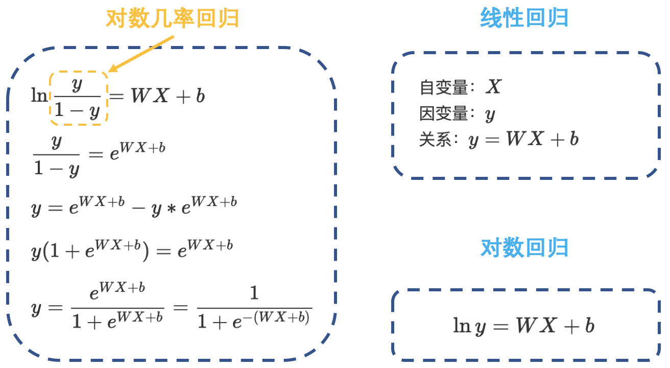
2. 逻辑回归
逻辑回归 (Logistic Regression) 是 线性 的 二分类 模型。
模型表达式:
\[y=f(WX+b)\] \[f(x)=\dfrac{1}{1+e^{-x}}\]即:
\[y=\dfrac{1}{1+e^{-(WX+b)}}\]这里,我们将 $f(x)$ 称为 Sigmoid 函数,又称 Logistic 函数:
\[\text{class}=\begin{cases}0, & y< 0.5 \\[2ex] 1, & y \ge 0.5 \end{cases}\]
线性回归是分析 自变量 $x$ 与 因变量 $y$ (标量) 之间关系的方法;而逻辑回归是分析 自变量 $x$ 与 因变量 $y$ (概率) 之间关系的方法。
机器学习训练的 5 个步骤:

- 数据:数据收集、清洗、划分、预处理。
- 模型:根据任务的难易程度,选择简单的线性模型或者复杂的神经网络模型等等。
- 损失函数:根据不同任务选择不同的损失函数并计算其梯度。例如:在线性回归中,我们可以选择均方误差损失函数;在分类任务中,我们可以选择交叉熵损失函数。
- 优化器:得到梯度之后,我们选择某种优化器来更新权值。
- 迭代训练:有了数据、模型、损失函数和优化器之后,我们就可以进行迭代训练了。
代码示例:
1
2
3
4
5
6
7
8
9
10
11
12
13
14
15
16
17
18
19
20
21
22
23
24
25
26
27
28
29
30
31
32
33
34
35
36
37
38
39
40
41
42
43
44
45
46
47
48
49
50
51
52
53
54
55
56
57
58
59
60
61
62
63
64
65
66
67
68
69
70
71
72
73
74
75
76
77
78
79
80
81
82
83
84
85
import torch
import torch.nn as nn
import matplotlib.pyplot as plt
import numpy as np
torch.manual_seed(10)

# ============================== Step 1/5: 生成数据 ===================================
sample_nums = 100
mean_value = 1.7
bias = 1
n_data = torch.ones(sample_nums, 2)
x0 = torch.normal(mean_value * n_data, 1) + bias    # 类别0 数据 shape=(100, 2)
y0 = torch.zeros(sample_nums)                       # 类别0 标签 shape=(100, 1)
x1 = torch.normal(-mean_value * n_data, 1) + bias   # 类别1 数据 shape=(100, 2)
y1 = torch.ones(sample_nums)                        # 类别1 标签 shape=(100, 1)
train_x = torch.cat((x0, x1), 0)
train_y = torch.cat((y0, y1), 0)


# ============================== Step 2/5: 选择模型 ===================================
class LR(nn.Module):
    def __init__(self):
        super(LR, self).__init__()
        self.features = nn.Linear(2, 1)
        self.sigmoid = nn.Sigmoid()

    def forward(self, x):
        x = self.features(x)
        x = self.sigmoid(x)
        return x


lr_net = LR()   # 实例化逻辑回归模型

# ============================== Step 3/5: 选择损失函数 ================================
loss_fn = nn.BCELoss()  # 二分类交叉熵损失 Binary Cross Entropy Loss

# ============================== Step 4/5: 选择优化器 ==================================
lr = 0.01   # 学习率
optimizer = torch.optim.SGD(lr_net.parameters(), lr=lr, momentum=0.9)    # 随机梯度下降

# ============================== Step 5/5: 模型训练 ====================================
for iteration in range(1000):

    # 前向传播
    y_pred = lr_net(train_x)

    # 计算 loss
    loss = loss_fn(y_pred.squeeze(), train_y)

    # 反向传播
    loss.backward()

    # 更新参数
    optimizer.step()

    # 绘图
    if iteration % 20 == 0:

        mask = y_pred.ge(0.5).float().squeeze()  # 以 0.5 为阈值进行分类
        correct = (mask == train_y).sum()   # 计算正确预测的样本个数
        acc = correct.item() / train_y.size(0)   # 计算分类准确率

        plt.scatter(x0.data.numpy()[:, 0], x0.data.numpy()[:, 1], c='r', label='class 0')
        plt.scatter(x1.data.numpy()[:, 0], x1.data.numpy()[:, 1], c='b', label='class 1')

        w0, w1 = lr_net.features.weight[0]
        w0, w1 = float(w0.item()), float(w1.item())
        plot_b = float(lr_net.features.bias[0].item())
        plot_x = np.arange(-6, 6, 0.1)
        plot_y = (-w0 * plot_x - plot_b) / w1

        plt.xlim(-5, 7)
        plt.ylim(-7, 7)
        plt.plot(plot_x, plot_y)

        plt.text(-5, 5, 'Loss=%.4f' % loss.data.numpy(), fontdict={'size': 20, 'color': 'red'})
        plt.title("Iteration: {}\nw0:{:.2f} w1:{:.2f} b:{:.2f} accuracy:{:.2%}".format(iteration, w0, w1, plot_b, acc))
        plt.legend()

        plt.show()
        plt.pause(0.5)

        if acc > 0.99:
            break
3. 总结
本节课介绍了 PyTorch 自动求导系统中的 torch.autograd.backward 和 torch.autograd.grad 这两个常用方法,并演示了一阶、二阶导数的求导过程;理解了自动求导系统,以及数据载体 —— 张量,前向传播构建计算图,计算图求取梯度过程。有了这些知识之后,我们就可以开始正式训练机器学习模型。这里通过演示逻辑回归模型的训练,学习了机器学习回归模型的五大模块:数据、模型、损失函数、优化器和迭代训练过程。这五大模块将是后面学习的主线。
下节内容:数据读取机制:Dataloader 与 Dataset
本作品采用知识共享署名-非商业性使用-相同方式共享 4.0 国际许可协议进行许可。 欢迎转载,并请注明来自:YEY 的博客 同时保持文章内容的完整和以上声明信息!