Lecture 15 损失函数 (一)

在前几节课中，我们学习了模型模块中的一些知识，包括如何构建模型以及怎样进行模型初始化。本节课我们将开始学习损失函数模块。

1. 损失函数的概念

损失函数 (Loss Function)：衡量模型输出与真实标签之间的差异。

下面是一个一元线性回归的拟合过程示意图：

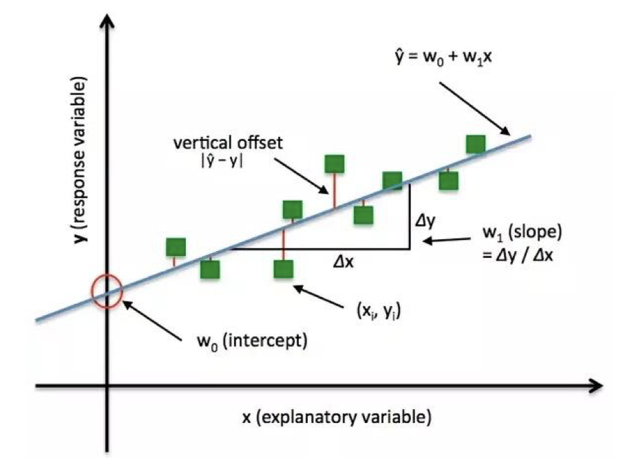
图中的绿色方块代表训练样本点 $(x_i, y_i)$，蓝色直线代表训练得到的模型 $\hat y = w_0 + w_1 x$，其中，$w_0$ 代表截距，$w_1 = \Delta y / \Delta x$ 代表斜率。可以看到，模型并没有完美地拟合每一个数据点，所以数据点和模型之间存在一个 损失 (Loss)，这里我们采用垂直方向上模型输出与真实数据点之差的绝对值 $|\hat y -y|$ 作为损失函数的度量。

另外，当我们谈到损失函数时，经常会涉及到以下三个概念：

损失函数 (Loss Function)：计算单个样本的差异。
\[\mathrm{Loss} = f(\hat y, y)\]
代价函数 (Cost Function)：计算整个训练集 $\mathrm{Loss}$ 的平均值。
\[\mathrm{Cost} = \dfrac{1}{n}\sum_{i=1}^{n} f(\hat y_i, y_i)\]
目标函数 (Objective Function)：最终需要优化的目标，通常包含代价函数和正则项。
\[\mathrm{Obj} = \mathrm{Cost} + \mathrm{Regularization}\]

注意，代价函数并不是越小越好，因为存在过拟合的风险。所以我们需要加上一些约束 (即正则项) 来防止模型变得过于复杂而导致过拟合，常用的有 L1 和 L2 正则项。因此，代价函数和正则项最终构成了我们的目标函数。

下面我们来看一下 PyTorch 中的 _Loss 类：

class _Loss(Module):
    def __init__(self, size_average=None, reduce=None, reduction='mean'):
        super(_Loss, self).__init__()
        if size_average is not None or reduce is not None:
            self.reduction = _Reduction.legacy_get_string(size_average, reduce)
        else:
            self.reduction = reduction

可以看到，_Loss 是继承于 Module 类的，所以从某种程度上我们可以将 _Loss 也视为一个网络层。它的初始化函数中主要有 3 个参数，其中 size_average 和 reduce 这两个参数即将在后续版本中被舍弃，因为 reduction 参数已经可以实现前两者的功能。

2. 交叉熵损失函数

在分类任务中，我们经常采用的是交叉熵损失函数。在分类任务中我们常常需要计算不同类别的概率值，所以交叉熵可以用来衡量两个概率分布之间的差异，交叉熵值越低说明两个概率分布越接近。

那么为什么交叉熵值越低，两个概率分布越接近呢？这需要从它与信息熵和相对熵之间的关系说起：

交叉熵 $=$ 信息熵 $+$ 相对熵

我们先来看最基本的 熵 (Entropy) 的概念：熵准确来说应该叫做 信息熵 (Information Entropy)，它是由信息论之父香农从热力学中借鉴过来的一个概念，用于描述某个事件的不确定性：某个事件不确定性越高，它的熵就越大。例如：“明天下雨” 这一事件要比 “明天太阳会升起” 这一事件的熵大得多，因为前者的不确定性较高。这里我们需要引入 自信息 的概念。

自信息 (Self-information)：用于衡量单个事件的不确定性。
\[I(X) = -\log [P(X)]\]
其中，$P(X)$ 为事件 $X$ 的概率。
熵 (Entropy)：自信息的期望，用于描述整个概率分布的不确定性。事件的不确定性越高，它的熵就越大。
\[H(P) = \mathrm{E}_{X\sim P}[I(X)] = \sum_{i=1}^{n}P(x_i)\log P(x_i)\]

为了更好地理解熵与事件不确定性的关系，我们来看一个示意图：

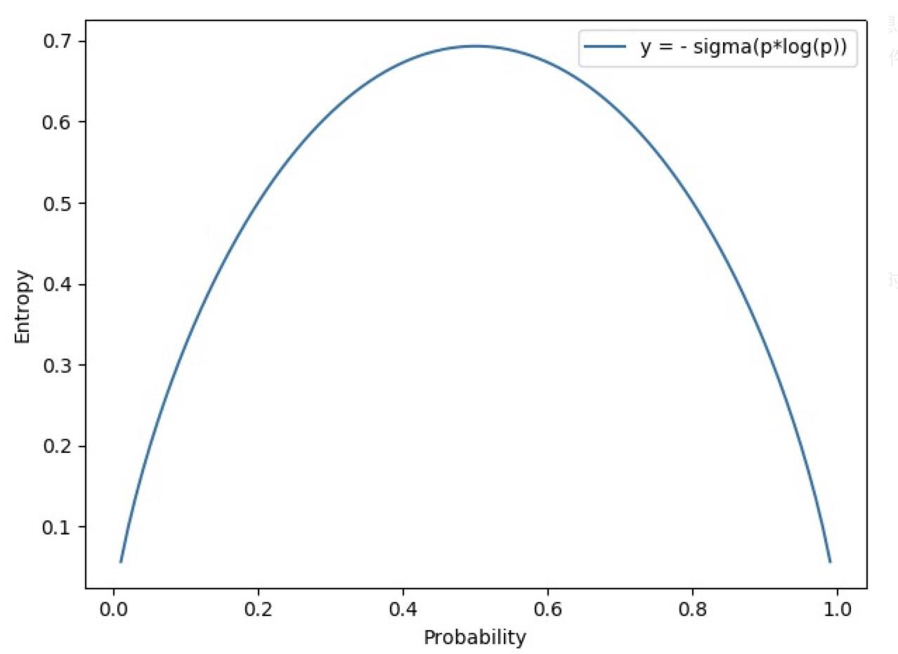
上面是伯努利分布 (两点分布) 的信息熵，可以看到，当事件概率为 $0.5$ 时，它的信息熵最大，大约在 $0.69$ 附近，即此时该事件的不确定性是最大的。注意，这里的 $0.69$ 是在二分类模型训练过程中经常会碰到的一个 Loss 值：有时在模型训练出问题时，无论我们如何进行迭代，模型的 Loss 值始终恒定在 $0.69$；或者在模型刚初始化完成第一次迭代后，其 Loss 值也很可能是 $0.69$，这表明我们的模型当前是不具备任何判别能力的，因为其对于两个类别中的任何一个都认为概率是 $0.5$。

下面我们来看一下相对熵的概念：

相对熵 (Relative Entropy)：又称 KL 散度 (Kullback-Leibler Divergence, KLD)，用于衡量两个概率分布之间的差异 (或者说距离)。注意，虽然 KL 散度可以衡量两个分布之间的距离，但它本身并不是一个距离函数，因为距离函数具有对称性，即 $P$ 到 $Q$ 的距离必须等于 $Q$ 到 $P$ 的距离，而相对熵不具备这种对称性。
\[D_{\mathrm{KL}}(P, Q) = \mathrm{E}_{X \sim P}\left[\log \dfrac{P(X)}{Q(X)}\right]\]
其中，$P$ 是数据的真实分布，$Q$ 是模型拟合的分布，二者定义在相同的概率空间上。我们需要用拟合分布 $Q$ 去逼近真实分布 $P$，所以相对熵不具备对称性。

下面我们再来看一下交叉熵的公式：

交叉熵 (Cross Entropy)：用于衡量两个分布之间的相似度。
\[H(P,Q)= -\sum_{i=1}^{n}P(x_i)\log Q(x_i)\]

下面我们对相对熵的公式进行展开推导变换，来观察一下相对熵与信息熵和交叉熵之间的关系：

\[\begin{aligned} D_{\mathrm{KL}}(P, Q) &= \mathrm{E}_{X \sim P}\left[\log \dfrac{P(X)}{Q(X)}\right] \\[2ex] &= \mathrm{E}_{X \sim P} [\log P(X) - \log Q(X) ] \\[2ex] &= \sum_{i=1}^{n} P(x_i) [\log P(x_i) - \log Q(x_i) ] \\[2ex] &= \sum_{i=1}^{n} P(x_i) \log P(x_i) - \sum_{i=1}^{n} P(x_i) \log Q(x_i) \\[2ex] &= H(P, Q) - H(P) \end{aligned}\]

所以，交叉熵等于信息熵加上相对熵：

\[H(P, Q) = H(P) + D_{\mathrm{KL}}(P, Q)\]

这里，$P$ 为训练集中的样本分布，$Q$ 为模型给出的分布。所以在机器学习中，我们最小化交叉熵实际上等价于最小化相对熵，因为训练集是固定的，所以 $H(P)$ 在这里是一个常数。

`nn.CrossEntropyLoss`

功能：nn.LogSoftmax() 与 nn.NLLLoss() 结合，进行交叉熵计算。

nn.CrossEntropyLoss(
    weight=None,
    size_average=None,
    ignore_index=-100,
    reduce=None,
    reduction='mean'
)

主要参数：

weight：各类别的 loss 设置权值。
ignore_index：忽略某个类别，不计算其 loss。
reduction：计算模式，可为 none/sum/mean。
- none：逐个元素计算。
- sum：所有元素求和，返回标量。
- mean：加权平均，返回标量。

PyTorch 中 nn.CrossEntropyLoss 的交叉熵计算公式：

没有针对各类别 loss 设置权值的情况：
\[\mathrm{loss}(x, class) = -\log \left(\dfrac{\exp(x[class])}{\sum_j \exp(x[j])} \right) = -x[class] + \log \left(\sum_j \exp(x[j])\right)\]
对各类别 loss 设置权值的情况：
\[\mathrm{loss}(x, class) = \mathrm{weight}[class] \left(-x[class] + \log \left(\sum_j \exp(x[j])\right)\right)\]

注意，这里的计算过程和交叉熵公式存在一些差异：

\[H(P,Q)= -\sum_{i=1}^{n}P(x_i)\log Q(x_i)\]

因为这里我们已经将一个具体数据点取出，所以这里 $\Sigma$ 求和式不再需要，并且 $P(x_i)=1$，因此公式变为：

\[H(P,Q)= -\log Q(x_i)\]

然后，为了使输出概率在 $[0,1]$ 之间，PyTorch 在这里使用了一个 Softmax 函数对数据进行了归一化处理，使其落在一个正常的概率值范围内。

代码示例：

import torch
import torch.nn as nn
import numpy as np

# fake data
inputs = torch.tensor([[1, 2], [1, 3], [1, 3]], dtype=torch.float)
target = torch.tensor([0, 1, 1], dtype=torch.long)  # 注意 label 在这里必须设置为长整型

# ------------------------ CrossEntropy loss: reduction ----------------------
# def loss function
loss_f_none = nn.CrossEntropyLoss(weight=None, reduction='none')
loss_f_sum = nn.CrossEntropyLoss(weight=None, reduction='sum')
loss_f_mean = nn.CrossEntropyLoss(weight=None, reduction='mean')

# forward
loss_none = loss_f_none(inputs, target)
loss_sum = loss_f_sum(inputs, target)
loss_mean = loss_f_mean(inputs, target)

# view
print("Cross Entropy Loss:\n ", loss_none, loss_sum, loss_mean)

输出结果：

Cross Entropy Loss:
  tensor([1.3133, 0.1269, 0.1269]) tensor(1.5671) tensor(0.5224)

可以看到，reduction 参数项在 none 模式下，计算出的 3 个样本的 loss 值分别为 $1.3133$、$0.1269$ 和 $0.1269$；在 sum 模式下，计算出 3 个样本的 loss 之和为 $1.5671$；在 mean 模式下，计算出 3 个样本的 loss 平均为 $0.5224$。

下面我们以第一个样本的 loss 值为例，通过手动计算来验证一下我们前面推导出的公式的正确性：

\[\mathrm{loss}(x, class) = -x[class] + \log \left(\sum_j \exp(x[j])\right)\]

idx = 0

input_1 = inputs.detach().numpy()[idx]      # [1, 2]
target_1 = target.numpy()[idx]              # [0]

# 第一项
x_class = input_1[target_1]

# 第二项
sigma_exp_x = np.sum(list(map(np.exp, input_1)))
log_sigma_exp_x = np.log(sigma_exp_x)

# 输出loss
loss_1 = -x_class + log_sigma_exp_x

print("第一个样本的 loss 为: ", loss_1)

输出结果：

第一个样本的 loss 为:  1.3132617

下面我们来看一下针对各类别 loss 设置权值的情况：

# def loss function
# 向量长度应该与类别数量一致，如果 reduction 参数为 'mean'，那么我们不需要关注
# weight 的尺度，只需要关注各类别的 weight 比例即可。
weights = torch.tensor([1, 2], dtype=torch.float)
# weights = torch.tensor([0.7, 0.3], dtype=torch.float)

loss_f_none_w = nn.CrossEntropyLoss(weight=weights, reduction='none')
loss_f_sum = nn.CrossEntropyLoss(weight=weights, reduction='sum')
loss_f_mean = nn.CrossEntropyLoss(weight=weights, reduction='mean')

# forward
loss_none_w = loss_f_none_w(inputs, target)
loss_sum = loss_f_sum(inputs, target)
loss_mean = loss_f_mean(inputs, target)

# view
print("\nweights: ", weights)
print(loss_none_w, loss_sum, loss_mean)

输出结果：

weights:  tensor([1., 2.])
tensor([1.3133, 0.2539, 0.2539]) tensor(1.8210) tensor(0.3642)

对比之前没有设置权值的结果，我们发现，在 none 模式下，由于第一个样本类别为 0，而其权值为 $1$，所以结果和之前一样，都是 $1.3133$。而第二个和第三个样本类别为 $1$，权值为 $2$，所以这里的 loss 是之前的 $2$ 倍，即 $0.2539$。对于 sum 模式，其结果为三个样本的 loss 之和，即 $1.8210$。而对于 mean 模式，现在不再是简单地将三个 loss 相加求平均，而是采用了加权平均的计算方式：因为第一个样本权值为 $1$，第二个和第三个样本权值都是 $2$，所以一共有 $1+2+2=5$ 份，loss 的加权均值为 $1.8210 / 5 = 0.3642$。

下面我们通过手动计算来验证在设置权值的情况下，mean 模式下的 loss 计算方式是否正确：

weights = torch.tensor([1, 2], dtype=torch.float)
weights_all = np.sum(list(map(lambda x: weights.numpy()[x], target.numpy())))

mean = 0
loss_sep = loss_none.detach().numpy()

for i in range(target.shape[0]):
    x_class = target.numpy()[i]
    tmp = loss_sep[i] * (weights.numpy()[x_class] / weights_all)
    mean += tmp

print(mean)

输出结果：

0.3641947731375694

可以看到，手动计算的结果和 PyTorch 中自动求取的结果一致，所以对于设置权值的情况，mean 模式下的 loss 不是简单的求和之后除以样本个数，而是除以权值的份数，即实际计算的是加权均值。

3. NLL/BCE/BCEWithLogits Loss

`nn.NLLLoss`

功能：实现负对数似然函数中的 负号功能。

nn.NLLLoss(
    weight=None,
    size_average=None,
    ignore_index=-100,
    reduce=None,
    reduction='mean'
)

主要参数：

weight：各类别的 loss 设置权值。
ignore_index：忽略某个类别。
reduction：计算模式，可为 none/sum/mean。
- none：逐个元素计算。
- sum：所有元素求和，返回标量。
- mean：加权平均，返回标量。

计算公式：

\[\ell(x,y) = L = \{l_1,\dots,l_N\}^{\mathrm T}\;,\qquad l_n = -w_{y_n}x_{n,y_n}\]

代码示例：

# fake data, 这里我们使用的还是之前的数据，注意 label 在这里必须设置为 long
inputs = torch.tensor([[1, 2], [1, 3], [1, 3]], dtype=torch.float)
target = torch.tensor([0, 1, 1], dtype=torch.long)

# weights
weights = torch.tensor([1, 1], dtype=torch.float)

# NLL loss
loss_f_none_w = nn.NLLLoss(weight=weights, reduction='none')
loss_f_sum = nn.NLLLoss(weight=weights, reduction='sum')
loss_f_mean = nn.NLLLoss(weight=weights, reduction='mean')

# forward
loss_none_w = loss_f_none_w(inputs, target)
loss_sum = loss_f_sum(inputs, target)
loss_mean = loss_f_mean(inputs, target)

# view
print("\nweights: ", weights)
print("NLL Loss", loss_none_w, loss_sum, loss_mean)

输出结果：

weights:  tensor([1., 1.])
NLL Loss tensor([-1., -3., -3.]) tensor(-7.) tensor(-2.3333)

注意，这里 nn.NLLLoss 实际上只是实现了一个负号的功能。对于 none 模式：这里第一个样本是第 0 类，所以我们这里只对第一个神经元进行计算，取负号得到 NLL Loss 为 $-1$；第二个样本是第 1 类，我们对第二个神经元进行计算，取负号得到 NLL Loss 为 $-3$；第三个样本也是第 1 类，我们对第二个神经元进行计算，取负号得到 NLL Loss 为 $-3$。对于 sum 模式，将三个样本的 NLL Loss 求和，得到 $-7$。对于 mean 模式，将三个样本的 NLL Loss 加权平均，得到 $-2.3333$。

`nn.BCELoss`

功能：二分类交叉熵。

nn.BCELoss(
    weight=None,
    size_average=None,
    reduce=None,
    reduction='mean'
)

主要参数：

weight：各类别的 loss 设置权值。
ignore_index：忽略某个类别。
reduction：计算模式，可为 none/sum/mean。
- none：逐个元素计算。
- sum：所有元素求和，返回标量。
- mean：加权平均，返回标量。

计算公式：

\[l_n = -w_n [y_n \cdot \log x_n + (1- y_n) \cdot \log(1-x_n)]\]

注意事项：由于交叉熵是衡量两个概率分布之间的差异，因此输入值取值必须在 $[0, 1]$。

代码示例：

# fake data, 这里我们设置 4 个样本，注意 label 在这里必须设置为 float
inputs = torch.tensor([[1, 2], [2, 2], [3, 4], [4, 5]], dtype=torch.float)
target = torch.tensor([[1, 0], [1, 0], [0, 1], [0, 1]], dtype=torch.float)

target_bce = target

# itarget
inputs = torch.sigmoid(inputs)  # 利用 Sigmoid 函数将输入值压缩到 [0,1]

# weights
weights = torch.tensor([1, 1], dtype=torch.float)

# BCE loss
loss_f_none_w = nn.BCELoss(weight=weights, reduction='none')
loss_f_sum = nn.BCELoss(weight=weights, reduction='sum')
loss_f_mean = nn.BCELoss(weight=weights, reduction='mean')

# forward
loss_none_w = loss_f_none_w(inputs, target_bce)
loss_sum = loss_f_sum(inputs, target_bce)
loss_mean = loss_f_mean(inputs, target_bce)

# view
print("\nweights: ", weights)
print("BCE Loss", loss_none_w, loss_sum, loss_mean)

输出结果：

weights:  tensor([1., 1.])
BCE Loss tensor([[0.3133, 2.1269],
        [0.1269, 2.1269],
        [3.0486, 0.0181],
        [4.0181, 0.0067]]) tensor(11.7856) tensor(1.4732)

由于这里我们有 4 个样本，每个样本有 2 个神经元，因此在 none 模式下我们这里得到 8 个 loss，即每一个神经元会一一对应地计算 loss。而 sum 模式就是简单地将这 8 个 loss 进行相加，mean 模式就是对这 8 个 loss 求加权均值。

下面我们通过手动计算来验证第一个神经元的 BCE loss 值是否等于 $0.3133$：

idx = 0

x_i = inputs.detach().numpy()[idx, idx]  # 获取第一个神经元的输出值
y_i = target.numpy()[idx, idx]  # 获取第一个神经元的标签

# loss
# l_i = -[ y_i * np.log(x_i) + (1-y_i) * np.log(1-y_i) ]      # np.log(0) = nan
l_i = -y_i * np.log(x_i) if y_i else -(1-y_i) * np.log(1-x_i)

# 输出loss
print("BCE inputs: ", inputs)
print("第一个 loss 为: ", l_i)

输出结果：

BCE inputs:  tensor([[0.7311, 0.8808],
        [0.8808, 0.8808],
        [0.9526, 0.9820],
        [0.9820, 0.9933]])
第一个 loss 为:  0.31326166

可以看到，手动计算的结果与 PyTorch 中 nn.BCELoss 的计算结果一致。

`nn.BCEWithLogitsLoss`

功能：结合 Sigmoid 与二分类交叉熵。

nn.BCEWithLogitsLoss(
    weight=None,
    size_average=None,
    reduce=None,
    reduction='mean',
    pos_weight=None
)

主要参数：

pos_weight：正样本的权值，用于平衡正负样本。
- 例如：正样本有 100 个，负样本有 300 个，正负样本比例为 $1:3$。因此我们可以将该项设为 $3$，这样即等价于正负样本各 300 个。
weight：各类别的 loss 设置权值。
ignore_index：忽略某个类别。
reduction：计算模式，可为 none/sum/mean。
- none：逐个元素计算。
- sum：所有元素求和，返回标量。
- mean：加权平均，返回标量。

计算公式：

\[l_n = -w_n[y_n \cdot \log \sigma(x_n) + (1-y_n)\cdot \log (1-\sigma (x_n))]\]

注意事项：网络最后不加 Sigmoid 函数。

代码示例：

inputs = torch.tensor([[1, 2], [2, 2], [3, 4], [4, 5]], dtype=torch.float)
target = torch.tensor([[1, 0], [1, 0], [0, 1], [0, 1]], dtype=torch.float)

target_bce = target

# inputs = torch.sigmoid(inputs)  # 这里增加 sigmoid 会使得计算不准确，因为相当于加了两层 sigmoid

weights = torch.tensor([1, 1], dtype=torch.float)

loss_f_none_w = nn.BCEWithLogitsLoss(weight=weights, reduction='none')
loss_f_sum = nn.BCEWithLogitsLoss(weight=weights, reduction='sum')
loss_f_mean = nn.BCEWithLogitsLoss(weight=weights, reduction='mean')

# forward
loss_none_w = loss_f_none_w(inputs, target_bce)
loss_sum = loss_f_sum(inputs, target_bce)
loss_mean = loss_f_mean(inputs, target_bce)

# view
print("\nweights: ", weights)
print(loss_none_w, loss_sum, loss_mean)

输出结果：

weights:  tensor([1., 1.])
tensor([[0.3133, 2.1269],
        [0.1269, 2.1269],
        [3.0486, 0.0181],
        [4.0181, 0.0067]]) tensor(11.7856) tensor(1.4732)

我们来看一下 pos_weight 的设置：

inputs = torch.tensor([[1, 2], [2, 2], [3, 4], [4, 5]], dtype=torch.float)
target = torch.tensor([[1, 0], [1, 0], [0, 1], [0, 1]], dtype=torch.float)

target_bce = target

weights = torch.tensor([1], dtype=torch.float)
pos_w = torch.tensor([1], dtype=torch.float)  # 将 pos_weight 设为 1 

loss_f_none_w = nn.BCEWithLogitsLoss(weight=weights, reduction='none', pos_weight=pos_w)
loss_f_sum = nn.BCEWithLogitsLoss(weight=weights, reduction='sum', pos_weight=pos_w)
loss_f_mean = nn.BCEWithLogitsLoss(weight=weights, reduction='mean', pos_weight=pos_w)

# forward
loss_none_w = loss_f_none_w(inputs, target_bce)
loss_sum = loss_f_sum(inputs, target_bce)
loss_mean = loss_f_mean(inputs, target_bce)

# view
print("\npos_weights: ", pos_w)
print(loss_none_w, loss_sum, loss_mean)

输出结果：

pos_weights:  tensor([1.])
tensor([[0.3133, 2.1269],
        [0.1269, 2.1269],
        [3.0486, 0.0181],
        [4.0181, 0.0067]]) tensor(11.7856) tensor(1.4732)

可以看到，当 pos_weight 设为 $1$ 时，计算的 loss 结果与之前一样。接下来我们将 pos_weight 改为 $3$ 来看一下结果会如何变化：

pos_w = torch.tensor([3], dtype=torch.float)  # 将 pos_weight 设为 3

输出结果：

pos_weights:  tensor([3.])
tensor([[0.9398, 2.1269],
        [0.3808, 2.1269],
        [3.0486, 0.0544],
        [4.0181, 0.0201]]) tensor(12.7158) tensor(1.5895)

可以看到，当 pos_weight 设为 $3$ 时，第一个样本 $[1,2]$ 的标签为 $[1,0]$，它的第一个神经元标签 $1$ 对应的 loss 变为了之前的 $3$ 倍，即 $0.3133 \times 3 = 0.9398$；第二个神经元标签 $0$ 对应的 loss 和之前一样，为 $2.1269$。其余三个样本的 loss 变化同理。

4. 总结

本节课中，我们学习了损失函数的概念，以及 4 种不同的损失函数。下节课中，我们将继续学习 PyTorch 中其余 14 种损失函数。

下节内容：损失函数 (二)

本作品采用知识共享署名-非商业性使用-相同方式共享 4.0 国际许可协议进行许可。欢迎转载，并请注明来自：YEY 的博客同时保持文章内容的完整和以上声明信息！

PyTorch 15：损失函数 (一)

PyTorch 学习笔记

Lecture 15 损失函数 (一)

1. 损失函数的概念

2. 交叉熵损失函数

`nn.CrossEntropyLoss`

3. NLL/BCE/BCEWithLogits Loss

`nn.NLLLoss`

`nn.BCELoss`

`nn.BCEWithLogitsLoss`

4. 总结

CATALOG

FEATURED TAGS

FRIENDS