Lecture 16 损失函数 (二)
上节课中,我们学习了损失函数的概念以及四种不同的损失函数。这节课我们继续学习 PyTorch 中提供的另外十四种损失函数。
1. PyTorch 中的损失函数
首先我们来看在回归任务中常用的两个损失函数 nn.L1Loss 和 nn.MSELoss:
nn.L1Loss
功能:计算 inputs 与 target 之差的绝对值。
1
2
3
4
5
nn.L1Loss(
    size_average=None,
    reduce=None,
    reduction='mean'
)
主要参数:
reduction:计算模式,可为none/sum/mean。none:逐个元素计算。sum:所有元素求和,返回标量。mean:加权平均,返回标量。
计算公式:
\[l_n = |x_n - y_n |\]nn.MSELoss
功能:计算 inputs 与 target 之差的平方。
1
2
3
4
5
nn.MSELoss(
    size_average=None,
    reduce=None,
    reduction='mean'
)
主要参数:
reduction:计算模式,可为none/sum/mean。none:逐个元素计算。sum:所有元素求和,返回标量。mean:加权平均,返回标量。
计算公式:
\[l_n = (x_n - y_n )^2\]代码示例:
1
2
3
4
5
6
7
8
9
10
11
12
13
14
15
16
17
18
19
20
21
22
import torch
import torch.nn as nn
import matplotlib.pyplot as plt
import numpy as np
from tools.common_tools import set_seed

set_seed(1)  # 设置随机种子

inputs = torch.ones((2, 2))
target = torch.ones((2, 2)) * 3

# ------------------------------------ L1 loss ----------------------------------
loss_f = nn.L1Loss(reduction='none')
loss = loss_f(inputs, target)

print("input:{}\ntarget:{}\nL1 loss:{}".format(inputs, target, loss))

# ------------------------------------ MSE loss ---------------------------------
loss_f_mse = nn.MSELoss(reduction='none')
loss_mse = loss_f_mse(inputs, target)

print("MSE loss:{}".format(loss_mse))
输出结果:
1
2
3
4
5
6
7
8
input:tensor([[1., 1.],
        [1., 1.]])
target:tensor([[3., 3.],
        [3., 3.]])
L1 loss:tensor([[2., 2.],
        [2., 2.]])
MSE loss:tensor([[4., 4.],
        [4., 4.]])
可以看到,这里我们的每个神经元的输入为 $x_i = 1$,输出为 $y_i=3$。所以,每个神经元的 L1 loss 为 $|x_i - y_i| = |1-3| = 2$,MSE loss 为 $(x_i - y_i)^2 = (1-3)^2 = 4$。
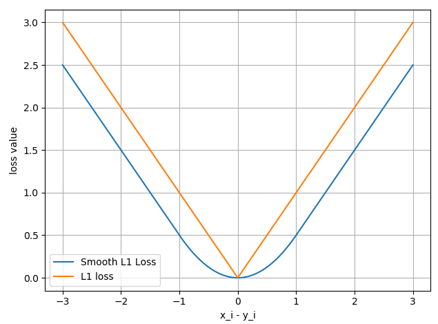
nn.SmoothL1Loss
功能:平滑的 L1 Loss,可以减轻离群点带来的影响。
1
2
3
4
5
nn.SmoothL1Loss(
    size_average=None,
    reduce=None,
    reduction='mean'
)
主要参数:
reduction:计算模式,可为none/sum/mean。none:逐个元素计算。sum:所有元素求和,返回标量。mean:加权平均,返回标量。
计算公式:
\[\mathrm{loss}(x,y) = \dfrac{1}{n}\sum_{i=1}^n z_i\]其中,
\[z_i = \begin{cases}0.5(x_i - y_i)^2\;, & \text{if } |x_i - y_i|< 1 \\[2ex] |x_i - y_i| - 0.5\;, & \text{otherwise}\end{cases}\]代码示例:
1
2
3
4
5
6
7
8
9
10
11
12
13
14
15
inputs = torch.linspace(-3, 3, steps=500)
target = torch.zeros_like(inputs)

loss_f = nn.SmoothL1Loss(reduction='none')
loss_smooth = loss_f(inputs, target)

loss_l1 = np.abs(inputs.numpy())

plt.plot(inputs.numpy(), loss_smooth.numpy(), label='Smooth L1 Loss')
plt.plot(inputs.numpy(), loss_l1, label='L1 loss')
plt.xlabel('x_i - y_i')
plt.ylabel('loss value')
plt.legend()
plt.grid()
plt.show()
输出结果:
PoissonNLLLoss
功能:泊松分布的负对数似然损失函数。
1
2
3
4
5
6
7
8
nn.PoissonNLLLoss(
    log_input=True,
    full=False,
    size_average=None,
    eps=1e-08,
    reduce=None,
    reduction='mean'
)
主要参数:
log_input:输入是否为对数形式,决定计算公式。full:计算所有 loss,默认为False。eps:修正项,避免input为 $0$ 时,log(input)为nan的情况。
计算公式:
-
当
\[\mathrm{loss}(x_n, y_n) = e^{x_n} - x_n \cdot y_n\]log_input=True时: -
当
\[\mathrm{loss}(x_n, y_n) = x_n - y_n \cdot \log(x_n + \mathrm{eps})\]log_input=False时:
代码示例:
1
2
3
4
5
6
7
inputs = torch.randn((2, 2))
target = torch.randn((2, 2))

loss_f = nn.PoissonNLLLoss(log_input=True, full=False, reduction='none')
loss = loss_f(inputs, target)

print("input:{}\ntarget:{}\nPoisson NLL loss:{}".format(inputs, target, loss))
输出结果:
1
2
3
4
5
6
input:tensor([[0.6614, 0.2669],
        [0.0617, 0.6213]])
target:tensor([[-0.4519, -0.1661],
        [-1.5228,  0.3817]])
Poisson NLL loss:tensor([[2.2363, 1.3503],
        [1.1575, 1.6242]])
下面我们以第一个神经元的 loss 为例,通过手动计算来验证我们前面的公式是否正确:
1
2
3
4
idx = 0
loss_1 = torch.exp(inputs[idx, idx]) - target[idx, idx]*inputs[idx, idx]

print("第一个元素的 loss 为:", loss_1)
输出结果:
1
第一个元素的 loss 为: tensor(2.2363)
可以看到,由于这里我们的 log_input=True,默认输入为对数形式,计算出的第一个神经元的 loss 为 $2.2363$,与前面 PyTorch 中 nn.PoissonNLLLoss 的计算结果一致。
nn.KLDivLoss
功能:计算 KL 散度 (KL divergence, KLD),即相对熵。
1
2
3
4
5
nn.KLDivLoss(
    size_average=None,
    reduce=None,
    reduction='mean'
)
主要参数:
reduction:计算模式,可为none/sum/mean/batchmean。none:逐个元素计算。sum:所有元素求和,返回标量。mean:加权平均,返回标量。batchmean:batchsize维度求平均值。
计算公式:
\[\begin{aligned} D_{\mathrm{KL}}(P,Q) = \mathrm{E}_{X\sim P}\left[\log \dfrac{P(X)}{Q(X)}\right] &= \mathrm{E}_{X\sim P}[\log P(X) - \log Q(X)] \\[2ex] &= \sum_{i=1}^{n} P(x_i)(\log P(x_i) - \log Q(x_i)) \end{aligned}\]其中,$P$ 为数据的真实分布,$Q$ 为模型拟合的分布。
PyTorch 中的计算公式:
\[l_n = y_n \cdot (\log y_n - x_n)\]由于 PyTorch 是逐个元素计算的,因此可以移除 $\Sigma$ 求和项。而括号中第二项这里是 $x_n$,而不是 $\log Q(x_n)$,因此我们需要提前计算输入的对数概率。
注意事项:需提前将输入计算 log-probabilities,例如通过 nn.logsoftmax() 计算。
代码示例:
1
2
3
4
5
6
7
8
9
10
11
12
13
inputs = torch.tensor([[0.5, 0.3, 0.2], [0.2, 0.3, 0.5]])
inputs_log = torch.log(inputs)
target = torch.tensor([[0.9, 0.05, 0.05], [0.1, 0.7, 0.2]], dtype=torch.float)

loss_f_none = nn.KLDivLoss(reduction='none')
loss_f_mean = nn.KLDivLoss(reduction='mean')
loss_f_bs_mean = nn.KLDivLoss(reduction='batchmean')

loss_none = loss_f_none(inputs, target)
loss_mean = loss_f_mean(inputs, target)
loss_bs_mean = loss_f_bs_mean(inputs, target)

print("loss_none:\n{}\nloss_mean:\n{}\nloss_bs_mean:\n{}".format(loss_none, loss_mean, loss_bs_mean))
输出结果:
1
2
3
4
5
6
7
loss_none:
tensor([[-0.5448, -0.1648, -0.1598],
        [-0.2503, -0.4597, -0.4219]])
loss_mean:
-0.3335360586643219
loss_bs_mean:
-1.000608205795288
由于我们的输入是一个 $2\times 3$ 的 Tensor,所以我们的 loss 也是一个 $2\times 3$ 的 Tensor。在 mean 模式下,我们得到 6 个 loss 的均值为 $-0.3335$;而 batchmean 模式下是 6 个 loss 相加再除以 $2$,所以得到 $-1.0006$。
下面我们以第一个神经元的 loss 为例,通过手动计算来验证 PyTorch 中的公式是否和我们之前提到的一致:
1
2
3
4
idx = 0
loss_1 = target[idx, idx] * (torch.log(target[idx, idx]) - inputs[idx, idx])  #  注意,这里括号中第二项没有取 log

print("第一个元素的 loss 为:", loss_1)
输出结果:
1
第一个元素的 loss 为: tensor(-0.5448)
可以看到,手动计算的结果与前面 PyTorch 中的 nn.KLDivLoss 的结果一致。
nn.MarginRankingLoss
功能:计算两个向量之间的相似度,用于 排序任务。该方法计算两组数据之间的差异,返回一个 $n\times n$ 的 loss 矩阵。
1
2
3
4
5
6
nn.MarginRankingLoss(
    margin=0.0,
    size_average=None,
    reduce=None,
    reduction='mean'
)
主要参数:
margin:边界值,$x_1$ 与 $x_2$ 之间的差异值。reduction:计算模式,可为none/sum/mean。
计算公式:
\[\mathrm{loss}(x,y)= \max (0, -y \cdot (x_1 - x_2) + \mathrm{margin})\]- 当 $y=1$ 时,我们希望 $x_1$ 比 $x_2$ 大,当 $x_1 > x_2$ 时, 不产生 loss。
- 当 $y=-1$ 时,我们希望 $x_2$ 比 $x_1$ 大,当 $x_2 > x_1$ 时,不产生 loss。
代码示例:
1
2
3
4
5
6
7
8
9
x1 = torch.tensor([[1], [2], [3]], dtype=torch.float)
x2 = torch.tensor([[2], [2], [2]], dtype=torch.float)

target = torch.tensor([1, 1, -1], dtype=torch.float)

loss_f_none = nn.MarginRankingLoss(margin=0, reduction='none')
loss = loss_f_none(x1, x2, target)

print(loss)
输出结果:
1
2
3
tensor([[1., 1., 0.],
        [0., 0., 0.],
        [0., 0., 1.]])
由于这里我们的输入是两个长度为 $3$ 的向量,所以输出的是一个 $3\times 3$ 的 loss 矩阵。该矩阵中的第一行是由 x1 中的第一个元素与 x2 中的三个元素计算得到的 loss。当 $y=1$ 时,$x_1 =1$,$x_2=2$,$x_1$ 并没有大于 $x_2$,因此会产生 loss 为 $\max (0, -1\times (1 - 2)) = 1$,所以输出矩阵中第一行的第一个元素为 $1$;第一行中的第二个元素同理。对于第一行中的第三个元素,$y = -1$,$x_1 =1$,$x_2=2$,满足 $x_2 > x_1$,因此不会产生 loss,即 loss 为 $\max (0, 1\times (1 - 2)) = 0$,所以输出矩阵中第一行的第三个元素为 $0$。
nn.MultiLabelMarginLoss
功能:多标签边界损失函数。例如四分类任务,样本 $x$ 属于第 $0$ 类和第 $3$ 类,注意这里标签为 $[0,3,-1,-1]$,而不是 $[1,0,0,1]$。
1
2
3
4
5
nn.MultiLabelMarginLoss(
    size_average=None,
    reduce=None,
    reduction='mean'
)
主要参数:
reduction:计算模式,可为none/sum/mean。
计算公式:
\[\mathrm{loss}(x,y) = \sum_{ij}\dfrac{\max(0, 1-x[ y [j] ] - x[i])}{x.\mathrm{size}(0)}\]其中,$i=0,\dots,x.\mathrm{size}(0)\;,\;j=0,\dots,y.\mathrm{size}(0)$,对于所有的 $i$ 和 $j$,都有 $y[j] \ge 0$ 并且 $i \ne y[j]$。
代码示例:
1
2
3
4
5
6
7
x = torch.tensor([[0.1, 0.2, 0.4, 0.8]])  # 一个四分类样本的输出概率
y = torch.tensor([[0, 3, -1, -1]], dtype=torch.long)  # 标签,该样本属于第 0 类和第 3 类

loss_f = nn.MultiLabelMarginLoss(reduction='none')
loss = loss_f(x, y)

print(loss)
输出结果:
1
tensor([0.8500])
下面我们通过手动计算来验证前面计算公式的正确性:
1
2
3
4
5
6
7
x = x[0]
item_1 = (1-(x[0] - x[1])) + (1 - (x[0] - x[2]))    # 第 0 类标签的 loss
item_2 = (1-(x[3] - x[1])) + (1 - (x[3] - x[2]))    # 第 3 类标签的 loss

loss_h = (item_1 + item_2) / x.shape[0]

print(loss_h)
输出结果:
1
tensor(0.8500)
可以看到,手动计算的结果与 PyTorch 中的 nn.MultiLabelMarginLoss 的结果一致。
nn.SoftMarginLoss
功能:计算二分类的 logistic 损失。
1
2
3
4
5
nn.SoftMarginLoss(
    size_average=None,
    reduce=None,
    reduction='mean'
)
主要参数:
reduction:计算模式,可为none/sum/mean。
计算公式:
\[\mathrm{loss}(x,y) = \sum_i \dfrac{\log(1 + \exp (-y[i] \cdot x[i]))}{x.\mathrm{nelement()}}\]其中,$x.\mathrm{nelement()}$ 为输入 $x$ 中的样本个数。注意这里 $y$ 也有 $1$ 和 $-1$ 两种模式。
代码示例:
1
2
3
4
5
6
7
inputs = torch.tensor([[0.3, 0.7], [0.5, 0.5]])  # 两个样本,两个神经元
target = torch.tensor([[-1, 1], [1, -1]], dtype=torch.float)  # 该 loss 为逐个神经元计算,需要为每个神经元单独设置标签

loss_f = nn.SoftMarginLoss(reduction='none')
loss = loss_f(inputs, target)

print("SoftMargin: ", loss)
输出结果:
1
2
SoftMargin:  tensor([[0.8544, 0.4032],
        [0.4741, 0.9741]])
下面我们以第一个神经元的 loss 为例,采用手动计算来验证上面公式的正确性:
1
2
3
4
5
6
7
idx = 0
inputs_i = inputs[idx, idx]
target_i = target[idx, idx]

loss_h = np.log(1 + np.exp(-target_i * inputs_i))

print(loss_h)
输出结果:
1
tensor(0.8544)
可以看到,手动计算的结果与 PyTorch 中的 nn.SoftMarginLoss 的结果一致。
nn.MultiLabelSoftMarginLoss
功能:SoftMarginLoss 的多标签版本。
1
2
3
4
5
nn.MultiLabelSoftMarginLoss(
    weight=None,
    size_average=None,
    reduce=None,
    reduction='mean')
主要参数:
weight:各类别的 loss 设置权值。reduction:计算模式,可为none/sum/mean。
计算公式:
\[\mathrm{loss}(x,y)= - \dfrac{1}{C} \cdot \sum_i y[i] \cdot \log\left(\dfrac{1}{1+\exp(-x[i]))} \right) + (1-y[i]) \cdot \log \left(\dfrac{\exp(-x[i])}{1+\exp(-x[i]))} \right)\]其中,$C$ 是标签类别的数量,$i$ 表示第 $i$ 个神经元,这里标签取值为 $0$ 或者 $1$,例如在一个四分类任务中,某样本标签为第 $0$ 类和第 $3$ 类,那么该样本的标签向量为 $[1,0,0,1]$。
代码示例:
1
2
3
4
5
6
7
inputs = torch.tensor([[0.3, 0.7, 0.8]])
target = torch.tensor([[0, 1, 1]], dtype=torch.float)

loss_f = nn.MultiLabelSoftMarginLoss(reduction='none')
loss = loss_f(inputs, target)

print("MultiLabel SoftMargin: ", loss)
输出结果:
1
MultiLabel SoftMargin:  tensor([0.5429])
下面我们通过手动计算验证上面公式的正确性:
1
2
3
4
5
6
7
i_0 = torch.log(torch.exp(-inputs[0, 0]) / (1 + torch.exp(-inputs[0, 0])))
i_1 = torch.log(1 / (1 + torch.exp(-inputs[0, 1])))
i_2 = torch.log(1 / (1 + torch.exp(-inputs[0, 2])))

loss_h = (i_0 + i_1 + i_2) / -3

print(loss_h)
输出结果:
1
tensor(0.5429)
可以看到,手动计算的结果与 PyTorch 中的 nn.MultiLabelSoftMarginLoss 的结果一致。
nn.MultiMarginLoss
功能:计算多分类的折页损失。
1
2
3
4
5
6
7
8
nn.MultiMarginLoss(
    p=1,
    margin=1.0,
    weight=None,
    size_average=None,
    reduce=None,
    reduction='mean'
)
主要参数:
p:可选1或2。weight:各类别的 loss 设置权值。margin:边界值。reduction:计算模式,可为none/sum/mean。
计算公式:
\[\mathrm{loss}(x,y) = \dfrac{\sum_i \max(0,\mathrm{margin}-x[y] + x[i])^p}{x.\mathrm{size(0)}}\]其中,$x\in \{0,\dots,x.\mathrm{size}(0)-1\}\;,\; y\in \{0,\dots,y.\mathrm{size}(0)-1\}$,并且对于所有的 $i$ 和 $j$,都有 $0 \le y[j] \le x.\mathrm{size}(0)-1$,以及 $i \ne y[j]$。
代码示例:
1
2
3
4
5
6
7
x = torch.tensor([[0.1, 0.2, 0.7], [0.2, 0.5, 0.3]])
y = torch.tensor([1, 2], dtype=torch.long)

loss_f = nn.MultiMarginLoss(reduction='none')
loss = loss_f(x, y)

print("Multi Margin Loss: ", loss)
输出结果:
1
Multi Margin Loss:  tensor([0.8000, 0.7000])
下面我们以第一个样本的 loss 为例,通过手动计算验证上面公式的正确性:
1
2
3
4
5
6
7
8
9
x = x[0]
margin = 1

i_0 = margin - (x[1] - x[0])
i_2 = margin - (x[1] - x[2])

loss_h = (i_0 + i_2) / x.shape[0]

print(loss_h)
输出结果:
1
tensor(0.8000)
可以看到,手动计算的结果与 PyTorch 中的 nn.MultiMarginLoss 的结果一致。
nn.TripletMarginLoss
功能:计算三元组损失,常用于人脸识别验证。
三元组损失:
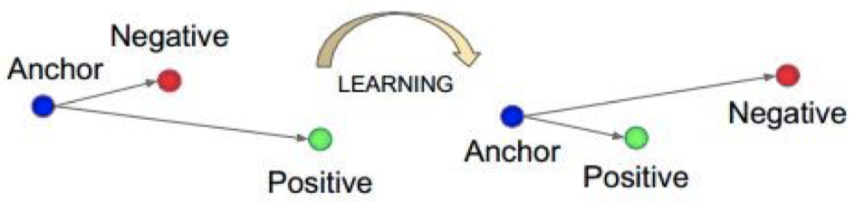
我们希望通过学习,使得 Anchor 与 Posttive 之间的距离小于 Anchor 与 Negative 之间的距离。
1
2
3
4
5
6
7
8
9
nn.TripletMarginLoss(
    margin=1.0,
    p=2.0,
    eps=1e-06,
    swap=False,
    size_average=None,
    reduce=None,
    reduction='mean'
)
主要参数:
p:范数的阶,默认为2。margin:边界值。reduction:计算模式,可为none/sum/mean。
计算公式:
\[L(a,p,n) = \max \{d(a_i, p_i) - d(a_i, n_i) + \mathrm{margin}, 0\}\]其中,$d(x_i, y_i) = \|\mathbf{x}_i - \mathbf{y}_i \|_p$。
代码示例:
1
2
3
4
5
6
7
8
anchor = torch.tensor([[1.]])
pos = torch.tensor([[2.]])
neg = torch.tensor([[0.5]])

loss_f = nn.TripletMarginLoss(margin=1.0, p=1)  # 范数为 1,即计算两者之差的绝对值
loss = loss_f(anchor, pos, neg)

print("Triplet Margin Loss", loss)
输出结果:
1
Triplet Margin Loss tensor(1.5000)
下面我们通过手动计算验证上面公式的正确性:
1
2
3
4
5
6
7
8
9
margin = 1
a, p, n = anchor[0], pos[0], neg[0]

d_ap = torch.abs(a-p)
d_an = torch.abs(a-n)

loss = d_ap - d_an + margin

print(loss)
输出结果:
1
tensor([1.5000])
可以看到,手动计算的结果与 PyTorch 中的 nn.TripletMarginLoss 的结果一致。
nn.HingeEmbeddingLoss
功能:计算两个输入的相似性,常用于非线性 embedding 和半监督学习。
1
2
3
4
5
6
nn.HingeEmbeddingLoss(
    margin=1.0,
    size_average=None,
    reduce=None,
    reduction='mean'
)
主要参数:
margin:边界值。reduction:计算模式,可为none/sum/mean。
计算公式:
\[l_n = \begin{cases}x_n\, , & \text{if } y_n = 1 \\[2ex] \max\{0,\Delta - x_n\}\, , & \text{if } y_n = -1\end{cases}\]注意事项:输入 $x$ 应为两个输入之差的绝对值。
代码示例:
1
2
3
4
5
6
7
inputs = torch.tensor([[1., 0.8, 0.5]])
target = torch.tensor([[1, 1, -1]])

loss_f = nn.HingeEmbeddingLoss(margin=1, reduction='none')
loss = loss_f(inputs, target)

print("Hinge Embedding Loss", loss)
输出结果:
1
Hinge Embedding Loss tensor([[1.0000, 0.8000, 0.5000]])
下面我们通过手动计算验证上面公式的正确性:
1
2
3
4
5
6
margin = 1.
loss_0 = inputs.numpy()[0, 0]
loss_1 = inputs.numpy()[0, 1]
loss_2 = max(0, margin - inputs.numpy()[0, 2])

print(loss_0, loss_1, loss_2)
输出结果:
1
1.0 0.8 0.5
可以看到,手动计算的结果与 PyTorch 中的 nn.HingeEmbeddingLoss 的结果一致。
nn.CosineEmbeddingLoss
功能:采用余弦相似度计算两个输入的相似性。
1
2
3
4
5
6
nn.CosineEmbeddingLoss(
    margin=0.0,
    size_average=None,
    reduce=None,
    reduction='mean'
)
主要参数:
margin:可取值 $[-1, 1]$,推荐为 $[0, 0.5]$。reduction:计算模式,可为none/sum/mean。
计算公式:
\[\mathrm{loss}(x,y) = \begin{cases}1-\cos(x_1,x_2)\, , & \text{if } y = 1 \\[2ex] \max\{0,\cos(x_1,x_2)-\mathrm{margin}\}\, , & \text{if } y = -1\end{cases}\]其中,
\[\cos(\theta) = \dfrac{A\cdot B}{\|A\| \|B\|} = \dfrac{\sum_{i=1}^{n}A_i \times B_i}{\sqrt{\sum_{i=1}^{n}(A_i)^2} \times \sqrt{\sum_{i=1}^{n}(B_i)^2}}\]代码示例:
1
2
3
4
5
6
7
8
x1 = torch.tensor([[0.3, 0.5, 0.7], [0.3, 0.5, 0.7]])
x2 = torch.tensor([[0.1, 0.3, 0.5], [0.1, 0.3, 0.5]])
target = torch.tensor([[1, -1]], dtype=torch.float)

loss_f = nn.CosineEmbeddingLoss(margin=0., reduction='none')
loss = loss_f(x1, x2, target)

print("Cosine Embedding Loss", loss)
输出结果:
1
Cosine Embedding Loss tensor([[0.0167, 0.9833]])
下面我们通过手动计算验证上面公式的正确性:
1
2
3
4
5
6
7
8
9
10
11
margin = 0.

def cosine(a, b):
    numerator = torch.dot(a, b)
    denominator = torch.norm(a, 2) * torch.norm(b, 2)
    return float(numerator/denominator)

l_1 = 1 - (cosine(x1[0], x2[0]))
l_2 = max(0, cosine(x1[0], x2[0]) - margin)

print(l_1, l_2)
输出结果:
1
0.016662120819091797 0.9833378791809082
可以看到,手动计算的结果与 PyTorch 中的 nn.CosineEmbeddingLoss 的结果一致。
nn.CTCLoss
功能:计算 CTC (Connectionist Temporal Classification) 损失,用于解决时序类数据的分类。
1
2
3
4
5
torch.nn.CTCLoss(
    blank=0,
    reduction='mean',
    zero_infinity=False
)
主要参数:
blank:blank label。zero_infinity:无穷大的值或梯度值为 $0$。reduction:计算模式,可为none/sum/mean。
代码示例:
1
2
3
4
5
6
7
8
9
10
11
12
13
14
15
16
17
18
19
T = 50      # Input sequence length
C = 20      # Number of classes (including blank)
N = 16      # Batch size
S = 30      # Target sequence length of longest target in batch
S_min = 10  # Minimum target length, for demonstration purposes

# Initialize random batch of input vectors, for *size = (T,N,C)
inputs = torch.randn(T, N, C).log_softmax(2).detach().requires_grad_()

# Initialize random batch of targets (0 = blank, 1:C = classes)
target = torch.randint(low=1, high=C, size=(N, S), dtype=torch.long)

input_lengths = torch.full(size=(N,), fill_value=T, dtype=torch.long)
target_lengths = torch.randint(low=S_min, high=S, size=(N,), dtype=torch.long)

ctc_loss = nn.CTCLoss()
loss = ctc_loss(inputs, target, input_lengths, target_lengths)

print("CTC loss: ", loss)
输出结果:
1
CTC loss:  tensor(7.5385, grad_fn=<MeanBackward0>)
2. 总结
到这里,我们已经学习完了 PyTorch 中的 18 种损失函数:
nn.CrossEntropyLossnn.NLLLossnn.BCELossnn.BCEWithLogitsLossnn.L1Lossnn.MSELossnn.SmoothL1Lossnn.PoissonNLLLossnn.KLDivLossnn.MarginRankingLossnn.MultiLabelMarginLossnn.SoftMarginLossnn.MultiLabelSoftMarginLossnn.MultiMarginLossnn.TripletMarginLossnn.HingeEmbeddingLossnn.CosineEmbeddingLossnn.CTCLoss
下节课中,我们将学习 PyTorch 中的优化器。
下节内容:优化器 (一)
本作品采用知识共享署名-非商业性使用-相同方式共享 4.0 国际许可协议进行许可。 欢迎转载,并请注明来自:YEY 的博客 同时保持文章内容的完整和以上声明信息!